11 Item Response Theory
This tutorial is adapted from 2 articles:
- MultiLCIRT: An R package for multidimensional latent class item response models
- Variable weighting via multidimensional IRT models in Composite Indicators construction
Thanks to Simone Del Sarto from University of Perugia, Italy for the guidance on this document.
11.1 Vulnerability as a “latent” variable
A major task in the measurement of complex and latent household vulnerability dimensions phenomena such as deprivation (or Basic Needs), wealth (or Coping capacity) and ability (or Well-being) consists of summarising information available from a set of dichotomous or ordinal questions (also referred as items) from an household survey questionnaire. For example:
Deprivation (or Basic Needs), is assessed by collecting data on the extent to which households possess certain commodities, engage in certain activities or are subject to financial pressures. The responses of individuals to deprivation item questionnaires constitute the manifest or observed indicators. (cf. Item response theory and the measurement of deprivation, Szeles and Fusco, 2013)
Wealth (or Coping capacity) is a latent concept to be derived from observable assets, and measures of wealth are calculated from a set of assets a household possesses (cf. Measuring Household Wealth with Latent Trait Modelling: An Application to Malawian DHS Data, Vandemoortele, 2014).
11.2 Building composite indicators with IRT
Item Response Theory (IRT) are specific type of statistical modeling that allows to address this complex challenge of building data-driven vulnerability scores without the use of proxy indicators. The assumptions that IRT approaches allows for are closer to the operational reality and needs:
Latent phenomenon → not directly observable through a proxy, meaning that vulnerability is not directly measurable .
Latent variable → assumed to have a discrete distribution rather than continuous vulnerability scales.
Phenomenon manifestation → response pattern to the items of a questionnaire rather to profile of respondents.
Summary of the phenomenon → composite indicators rather than predicted scores.
Item Response Theory (IRT) (also known as latent trait theory, strong true score theory, or modern mental test theory) is a paradigm for the design, analysis, and scoring of tests, questionnaires, and similar instruments measuring abilities, attitudes, or other latent variables. It is a theory of testing based on the relationship between individuals’ performances on a test item and the test takers’ levels of performance on an overall measure of the ability that item was designed to measure. IRT models the response of each respondant of a given ability to each item in the test.
The term item, here is generic, covering all kinds of informative items. They might be multiple choice questions that have incorrect and correct responses, but are also commonly statements on questionnaires that allow respondents to indicate level of agreement (a rating or Likert scale), or patient symptoms scored as present/absent, or diagnostic information in complex systems.
The main advantage of the discrete approach consists in the possibility of clustering the statistical units into homogeneous groups (latent classes): units (people, refugees and so on) in the same class share very similar characteristics in terms of the investigated (multidimensional) latent trait. Hence, this model would also allow us to classify refugees in similar groups. Such model can support prioritization needs as it assigns a score to each group, so that it is possible to highlight the most/least vulnerable groups of refugees and/or sketch several refugees’ profiles according to the various dimensions of it.
Composite indicators can be built using IRT using the following procedure:
- Step 1 : Assess dimensionality within the variables of the data-set → Multidimensional Latent Class IRT model + clustering algorithm
- Step 2 : Adoption the best model for assigning weights to the test items. This steps also allows to account for dimensionality (clusters) within respondents.
- Step 3 : Item aggregation using the weights obtained at the previous step → construction of a composite indicator for each dimension
11.2.1 Step 0: Data Preparation
Data are loaded in a data frame and converted in a matrix, corresponding to the unit-by-unit response configurations.
To make the further estimation of the proposed models and clustering of items faster perform the analyses after aggregating the original records which correspond to the same response pattern so as to obtain a matrix with a record for each distinct response configuration (rather than for each statistical unit).
The function function aggr_data is then applied to this matrix. Output from function is:
data_dis: matrix of distinct configurations → S (used after in model estimation);freq: vector of corresponding frequencies → yv (used after in model estimation);
label: index of each original response configuration among the distinct ones.
The data-set in this reports contains the responses of a sample of 201 / 201 records to 14 / 196 binary items.
Tableplot is a powerful visualization method to explore and analyse large multivariate datasets. The representation below are used to help in the understanding of the data, explore the relationships between the variables, discover strange data patterns, and check the occurrence and selectivity of missing values.
11.2.2 Step 1: Clustering algorithm / Dimensionality assessment
The first steps aims at grouping variables measuring the same latent construct in the same cluster
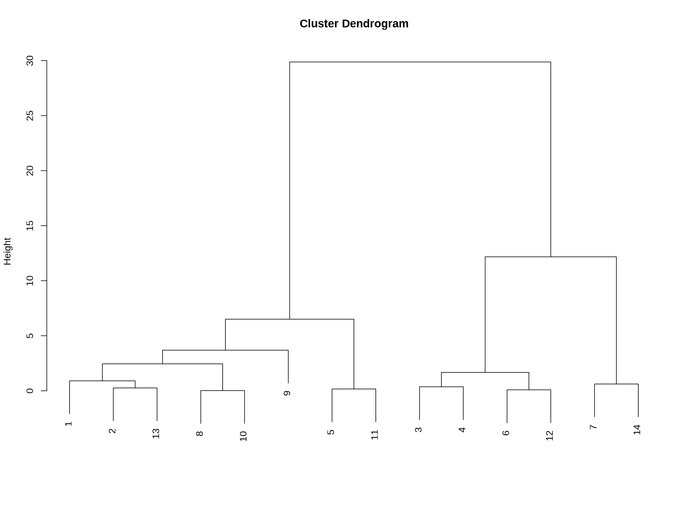
Investigating the best number of latent classes (parameter k) is done through Hierarchical clustering of items based on the Rasch model. The function class_item is used, it can take a long execution time. The classification is based on a sequence of likelihood ratio tests between pairs of multidimensional models suitably formulated.
The dendrogram below highlights three dimensions composing the multidimensional construct. Considering the item contents, the assessed dimension can be interpreted from a narrative point of view.

The following tables allows to interpret the clustering:
The first two columns (entitled
items) indicate items or groups collapsed at each step of the clustering procedure,the third column(
deviance) reports the corresponding LR statistic,the fourth column(
df)reports the number of degrees of freedom,the fifth (
p-value) reports the p-value, andthe last column (
newgroup) contains the new group of items that is formed at each step.
11.2.3 Step 2: Model selection
The second step is a selection procedure based on estimation of ordinal polytomous multidimensional LCIRT model. The formulation of a specific model in the class of multidimensional Latent Class (LC) IRT models univocally depends on:
- number of latent classes
k, - adopted parameterization in terms of
linkfunction , - constraints on the item parameters , and
- number of latent dimensions (
s) and the corresponding allocation of items within each dimension
Parameter estimation for multidimensional IRT models based on discreteness of latent traits is performed through function est_multi_poly requires the following main input:
S: matrix of all response sequences observed at least once in the sample and listed row-by-row. Usually,S is a matrix of type data_dis obtained by applying function aggr_data to the original data. Missing responses are allowed and they are coded as NaN;yv: vector of the frequencies of every response configuration in S corresponding to the output freq of function aggr_data (default value is given by a vector of ones, implying a unit weight for each record in S);k: number of latent classes - defined in the step 1;X: matrix of observed covariates, having the same dimension as S (default value is NULL, indicating the absence of covariates in the study);start: method of initialization of the algorithm: 0 ( = default value) for deterministic starting values, 1 for random starting values, and 2 for arguments given bytheuser. If start = 2 ,we also need to specify as input the initial values of weights, support points, and discriminating an ddifficulty item parameters (using additional input arguments that are set equal to NULL otherwise);link: type of link function: 0 (= default value) for the standard Latent Class model (i.e., no link function is specified),1 for global logits, and 2 for local logits. In the case of dichotomous responses, it is the same to specify link = 1 or link = 2;disc: indicator of constraints on the discriminating item parameters: 0 (= default value) if γj= 1, j=1 ,…, r, and 1 otherwise;difl: indicator of constraints on the difficulty item parameters: 0 (= default value) if difficulties are free and 1 if βjx= βj+ τxmulti: matrix with a number of rows equal to the number of dimensions and elements in each row equal to the indices of the items measuring the dimension corresponding to that row. Cases where dimensions are measured by a different number of items are allowed, and the number of columns of matrix multi corresponds to the number of items in the largest dimension.
Function est_multi_poly supplies the following output:
Piv: optional object of type matrix containing the estimated weights of thelatent classes subject-by-subject (the weights may be different across subjects in the presence of covariates);Th: estimated matrix of ability levels (support points) for each dimension (= row of matrix Th) and latent class (= column of matrix Th);Bec: estimated vector of difficulty item parameters (split in two vectors if difl = 1);gac: estimated vector of discriminating item parameters; if disc = 0 (Rasch-type model), all values of vector gac are constrained to 1;fv: vector indicating the reference item chosen for each latent dimension;Phi: optional object of type array containing the conditional response probabilities (see Eq.(1)) for every item and latent class. The array is made of as many matrices as the latent classes; moreover, the j -th column of each of such matrices refers to item j , where as the x-th row of each matrix refers to the x- th responsecategory(x = 0,…, lj − 1) of item j. In the case of items differing in the number of response categories, zeros are included in the corresponding cells;Pp: optional object of type matrix containing the posterior probabilities of belonging to latent class c (column c of the Pp matrix), given the response configuration (row of the Pp matrix);lk: log-likelihood at convergence of the EM algorithm;np: number of free parameters;aic: Akaike Information Criterion index (Akaike,1973);bic: Bayesian Information Criterion index (Schwarz,1978)
11.2.3.1 Number latent classes to consider
Checking here the optimal value of parameter k
| log-lik. | np | BIC | |
| model1 | -3,153.151 | 42 | 6,529.040 |
| model2 | -2,814.635 | 85 | 6,080.051 |
| model3 | -2,677.822 | 128 | 6,034.468 |
| model4 | -2,645.435 | 171 | 6,197.736 |
The model with lowest BIC is retained (i.e. k = 3).
11.2.3.2 Define parameterization on link function
To define if Global or local logit shall be used, we need to identify the optimal value of parameter link (1= Glocal logit, 2 = Local logit)
| log-lik. | np | BIC | |
| model1 | -2,726.348 | 72 | 5,834.534 |
| model2 | -2,741.321 | 72 | 5,864.479 |
The model with lowest BIC is retained (i.e. link = 1).
11.2.3.3 Constraints on the item parameters: Likelihood ratio
To test between nested multidimensional LC IRT models, we can compare different multidimensional model: a restricted model against a larger multidimensional model based on a higher number of dimensions.
A typical example is testing a unidimensional model (and then the hypothesis of unidimensionality) against a bidimensional model through function test_dim.
We will retain here the model with the smaller BIC value - Retained value for link = 1
11.2.3.4 Test of unidimensionality
Once the global logit has been chosen as the best link function, we carry on with the test of unidimensionality.
An LR test is used to comparemodels which differ in terms of the dimensional structure, all other elements being equal (i.e. free item discriminating and difficulty parameters), that is, * (i) a graded response model (GRM) with an r-dimensional structure, * (ii) a graded response model (GRM) with a bidimensional structure (i.e., anxiety and depression), as suggested by the structure of the questionnaire, and * (iii) a graded response model (GRM) with a unidimensional structure (i.e., all the items belong to the same dimension).
For this, models are calculated with different parameters:
* Difficulty levels (Free or Constrained, ie. constant or non-constant) difl.
* Discriminating indices (Free or Constrained, ie. constant or non-constant) disc.
| log-lik. | np | BIC | LR(vs. model1) | df | p-value | |
| model1 | -2,731.893 | 59 | 5,776.682 | |||
| model2 | -2,795.570 | 33 | 5,766.149 | 127.353 | 26 | 0 |
| model3 | -2,741.285 | 46 | 5,726.521 | 18.782 | 13 | 0.130 |
| log-lik. | np | BIC | LR(vs. model1) | df | p-value | |
| model1 | -2,741.285 | 46 | 5,726.521 | |||
| model2 | -2,844.518 | 20 | 5,795.102 | 206.467 | 26 | 0 |
| Class 1 | Class 2 | Class 3 | |
| Dimension 1 | -0.775 | 1.184 | 3.419 |
| prob | 0.342 | 0.491 | 0.167 |
11.2.4 Step 3: Items aggregation using the weights
The discrimination parameters express the informative capacity of a variable and its relative importance within sub-dimensions of the latent variables (as the model is multidimensional): so that the weight of a variable expresses the relative importance of that variable in the dimension it belongs to.
Weights are extracted from discrimination parameters, estimated through a Multidimensional IRT model, using a 2PL parametrisation
Two composite indicators can be calculated:
- Unweighted score (raw relative frequency of correct response)
- Weighted score, using ˆ γ j (and their transformation) for weighting the items
11.2.4.1 Multidimensional scores
gamma_hat: \(\hat{\gamma}_j\) (weights) from the model selected in the step above.
Since two dimensions are supposed, these weights can be divided into two groups
A useful thing to do is to rescale the parameters (within each dimension), so that the most discriminating item (for each dimension) has gamma_hat:\(\hat{\gamma}_j = 1\) and the other items have \(\hat{\gamma}_j < 1\). This is obtained by dividing each vector by its maximum element.
We can now use scaled discriminating item parameters parameters as weights.
Since these two sets of parameters are dimension-specific so they are not are not comparable.
Two different composite indicators can be constructed at this stage: one for the first dimension (dim1) and one for the second dimension (dim2).
Note that dividing by the weight sum (sum(gamma_hat1)) is not necessary, it depends on the type of indicator you need (in terms of sum or average).
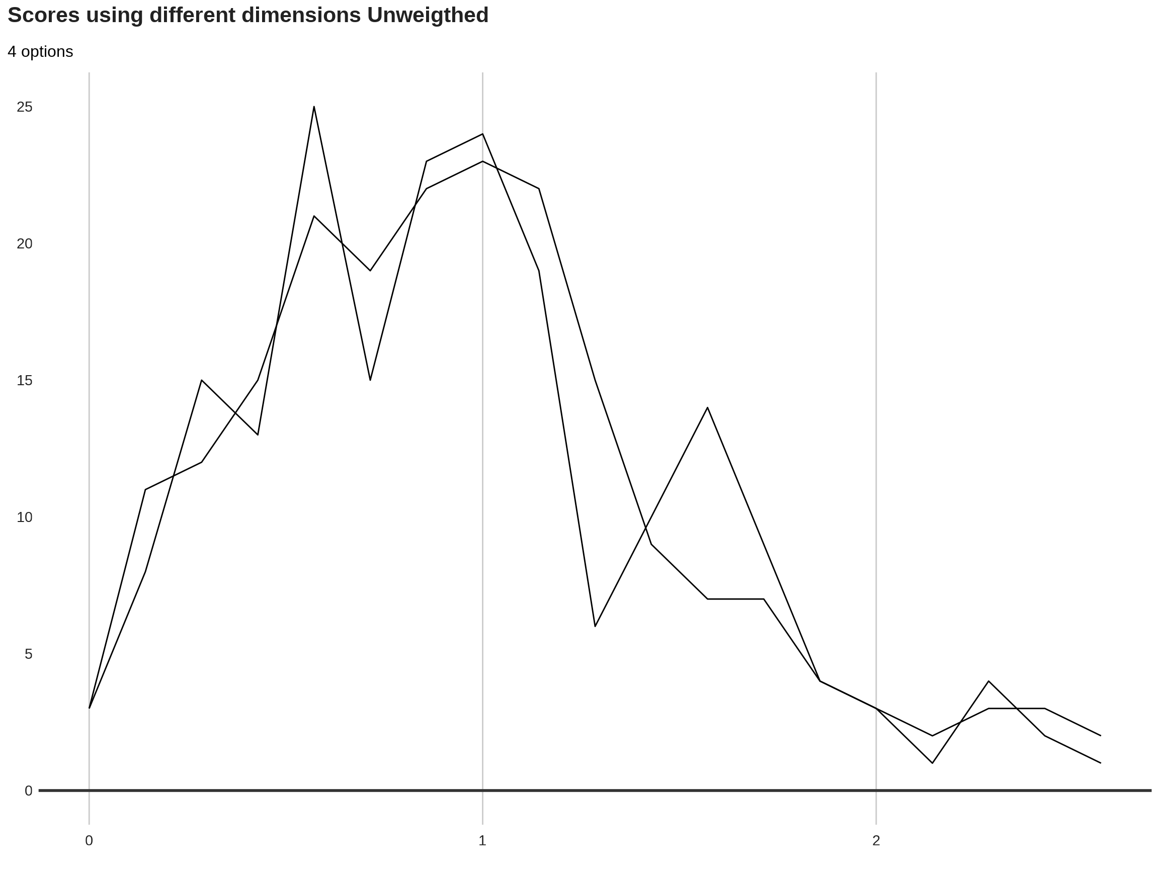
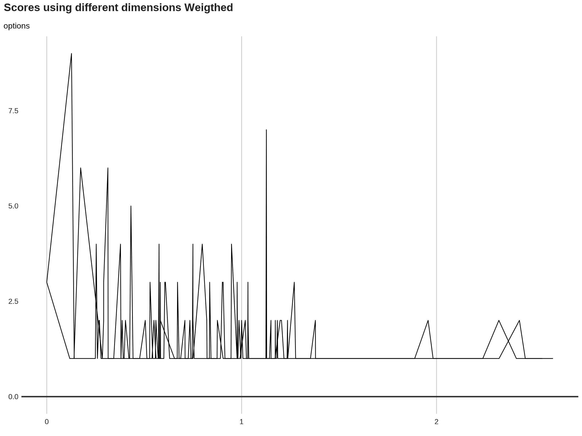
These indicators can be compared with the unweighted counterpart.
| CI1w | CI1unw | CI2w | CI2unw | |
| 1 | 1.127 | 1.143 | 1.173 | 1.143 |
| 2 | 0.576 | 0.571 | 0.715 | 0.714 |
| 3 | 1.379 | 1.429 | 0.873 | 0.857 |
| 4 | 0.671 | 0.714 | 0.576 | 0.571 |
| 5 | 0.279 | 0.286 | 0.432 | 0.429 |
| 6 | 0.549 | 0.571 | 0.432 | 0.429 |
Visualisation of resulting composite indicator


11.2.4.2 Sinle composite indicator
One wish to have a unique composite indicator, computed by using the entire response pattern of each unit.
In this case, the discrimination parameters need to be made comparable across dimensions. Then, we have to compute \(\gamma_j^*\).
First, we need to compute gamma_hat: \(\hat{\sigma}_d\)
Then, we can compute gamma_hat: \(\gamma_j^* = \hat{\sigma}_d \hat{\gamma}_j, j \in \mathcal{J}_d\).
As the standard deviation of the latent traits is taken into consideration, the item discriminations are now comparable.
For example, we could rank the items according to their discrimination.
Hence, a unique composite indicator can be built using these last weights.
Finally, one could rescale these last parameters (in order to obtain those denoted by \(w_j\) in the paper).
| item | discr | unique | |
| 3 | 7 | 0.867 | 0.830 |
| 14 | 14 | 1.003 | 0.764 |
| 7 | 12 | 1.016 | 0.811 |
| 12 | 9 | 1.119 | 0.804 |
| 1 | 2 | 1.128 | 1 |
| 2 | 6 | 1.145 | 0.775 |
| 10 | 4 | 1.188 | 0.587 |
| 9 | 3 | 1.199 | 0.813 |
| 4 | 8 | 1.201 | 0.758 |
| 5 | 10 | 1.213 | 0.821 |
| 8 | 1 | 1.226 | 0.969 |
| 13 | 13 | 1.281 | 0.688 |
| 6 | 11 | 1.432 | 0.867 |
| 11 | 5 | 1.477 | 0.679 |
If the data at issue are multilevel (e.g., refugees nested in different neighborhoods/villages/camps districts), the model can be extended to cluster high-level units (i.e. neighborhoods/villages/camps districts) as well. Further, covariates can be included to check the effects (if any) of individual (or higher level) covariates in the units’ class membership probabilities.
Additionally, Discrete Multidimensional Two-Tier IRT Model, an extension of the previous models can be explored to account for the double dependency of single items on more than one dimension of the Latent Variable.
In further research, the proposed procedure can therefore be extended through a classification of higher-order units in homogeneous groups - instead of ranking them one by one - that would take advantage of the latent class part of the described method, and account for the multilevel structure of the data. So basically not only the analysis would provide the vulnerability score of household but also account for a potential geographic effect within their vulnerability profile.
Another element of research includes to define the impact of sampling on the resulting weights.